3DGS
约 2609 个字 174 行代码 12 张图片 预计阅读时间 11 分钟
Abstract
 3DGS: 3D Gaussian Splatting for Real-Time Radiance Field Rendering
Idea
Introduction
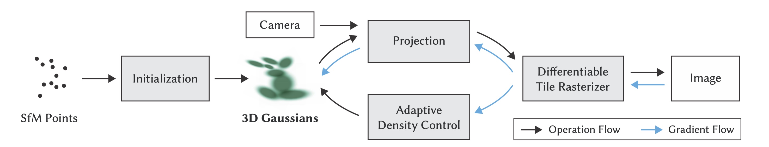
- 基于 Splatting 和机器学习的三维重建方法,用于实时且逼真地渲染从一组图像中学到的场景,改善 NeRF 的训练速度和渲染质量的瓶颈问题,保持有竞争力的训练时间的同时实现最先进的视觉质量,允许在 1080p 分辨率下实现高质量的实时( >= 30 fps)的新视图合成
- 3DGS 进行场景表达,多个高斯模型共同构成整个场景的连续体积表示
- 从最初由 SfM 生成的稀疏点开始初始化
- 3DGS 这种基元,继承可微分体积表示的属性,同时是非结构化和显式的,容易投影到 2D,快速 \(\alpha\)-blender
- 自适应密度控制优化:针对 3DGS 的各种属性 (位置、不透明度、各向异性协方差和球谐函数) 进行优化,且交错进行,包括在优化过程中移除 3DGS,以此精确表达场景
- 快速光栅化:使用高速 GPU,支持各向异性抛雪球,保证高质量实时渲染
Splatting
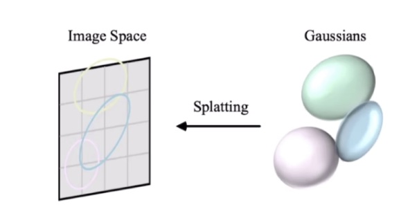
什么是 Splatting?什么是 3DGS?为什么选择 GS?
- 一种体渲染的方法(抛雪球法、足迹法、喷溅
) :从 3D 物体渲染到 2D 平面 - NeRF 是被动的,方式是
Ray-casting,计算出每个像素点收到发光粒子的影响来生成图像 - Splatting 是主动的,计算出每个发光粒子如何影响像素点
- 想象输入是一些雪球,图片是一面砖墙,图像生成过程是向墙面扔雪球的过程,每扔一个雪球,墙上都有扩散痕迹 footprint,流程:
- 选择雪球
- 抛掷雪球,从 3D 投影到 2D,得到足迹
- 合成,形成最后图像
选择雪球 3DGS 
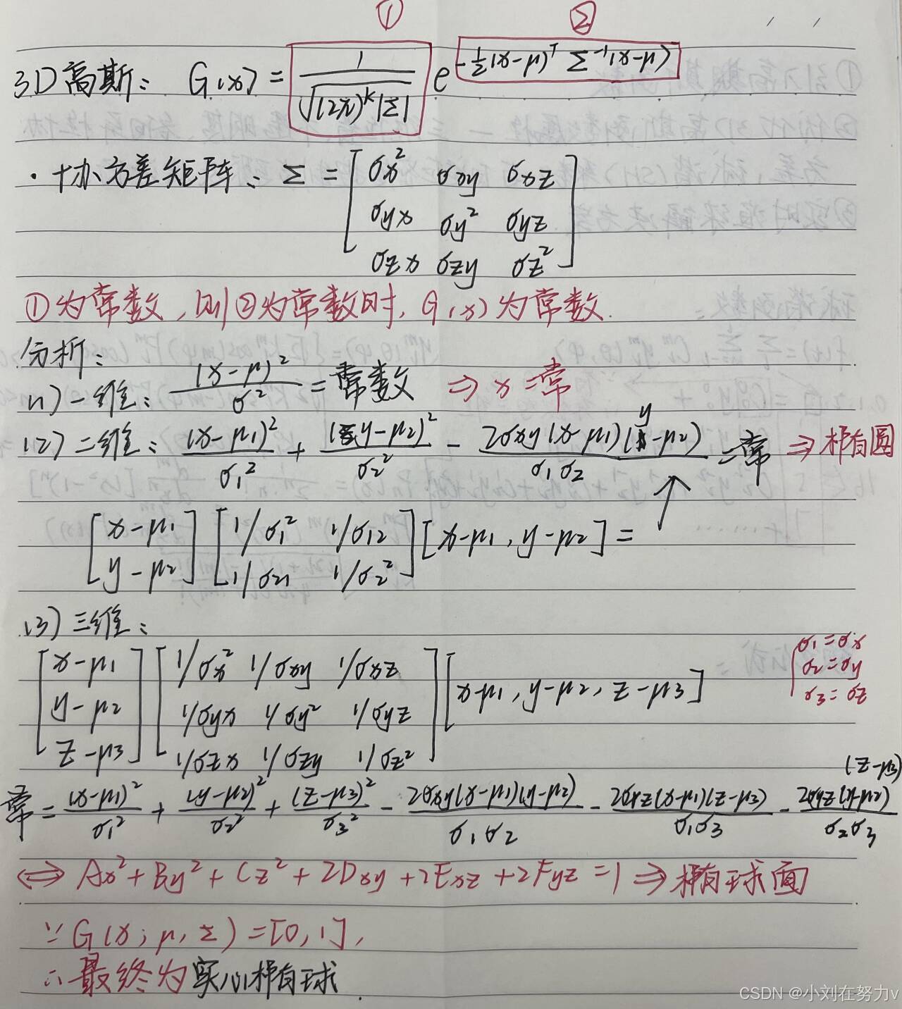
- 输入是点云,无体积,需要一个核进行膨胀,可以用高斯 / 圆 / 正方体 ...
- 选择高斯的理由,有很好的数学性质:
- 仿射变换后高斯核仍然闭合
- 3D 降到 2D 后(沿着某一轴积分)仍然是高斯
- 椭球高斯 \(G(x;\mu,\sum)=\frac{1}{\sqrt{(2\pi)^k \left | \sum \right |}} \exp^{-\frac{1}{2}(x-\mu)^\top\sum^{-1}(x-\mu)}\),\(\mu\) 表示均值,\(\sum\) 表示协方差矩阵,半正定(高维时从方差变成协方差矩阵)
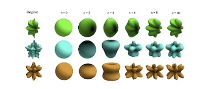
为什么 3DGS 是椭球?
各向同性和各向异性
-
各向同性
- 在所有方向具有相同的扩散程度(梯度
) ,例如球 - 3D 高斯分布:协方差矩阵是对角矩阵
\[ \sum = \begin{bmatrix} \sigma^2 & 0 &0 \\ 0 & \sigma^2 &0 \\ 0 & 0 & \sigma^2 \end{bmatrix} \] - 在所有方向具有相同的扩散程度(梯度
-
各向异性
- 在不同方向具有不同的扩散程度(梯度
) ,例如椭球 - 3D 高斯分布:协方差矩阵是对角矩阵
\[ \sum = \begin{bmatrix} \sigma_x^2 & \sigma_{xy} & \sigma_{xz} \\ \sigma_{yx} & \sigma_y^2 & \sigma_{yz} \\ \sigma_{zx} & \sigma_{zy} & \sigma_z^2 \end{bmatrix} \] - 在不同方向具有不同的扩散程度(梯度
3DGS 与协方差矩阵 
协方差矩阵和椭球有什么关系?为什么能控制椭球形状?
高斯分布的仿射变换:
- \(\mathcal{w}=A \mathcal{x} + b\)
- \(\mathcal{w} \thicksim N(A\mu+b, A\sum A^\top)\)
- \(\sum=A \cdot I \cdot A^\top\) 即任意高斯可以看作是标准高斯通过仿射变换得到
协方差矩阵为什么能用缩放和旋转矩阵表达?
\(A = RS\) \(\sum=A \cdot I \cdot A^\top = R \cdot S \cdot I \cdot (R \cdot S)^\top = R \cdot S \cdot S^\top \cdot R^\top\)
计算协方差矩阵 Code
# covariance = RS[S^T][R^T]
def computeCov3D(scale, mod, rot):
   # create scaling matrix
   S = np.array(
       [[scale[0] * mod, 0, 0], [0, scale[1] * mod, 0], [0, 0, scale[2] * mod]]
   )

   # normalize quaternion to get valid rotation
   # we use rotation matrix
   R = rot

   # compute 3d world covariance matrix Sigma
   M = np.dot(R, S)
   cov3D = np.dot(M, M.T)

   return cov3D
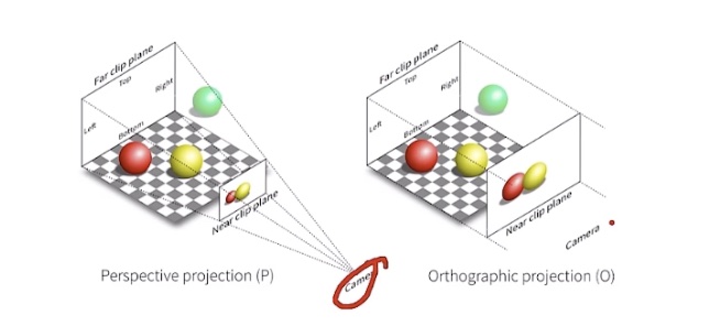
抛雪球 从 3D 到像素 
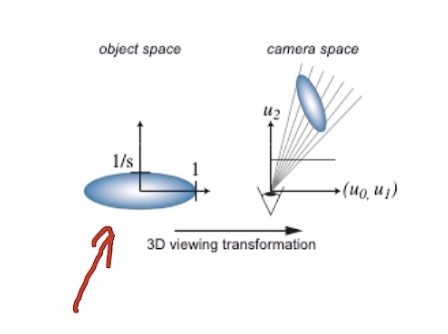
- 在相机模型中:世界坐标系、相机坐标系、归一化坐标系、像素坐标系
- 在 CG 中:观测变换、投影变换、视口变换、光栅化
观测变换、投影变换、视口变换、光栅化
-
观测变换:
- 从世界坐标系到相机坐标系
- 仿射变换
- \(\mathcal{w}=A \mathcal{x} + b\)
-
投影变换
- 3D 到 2D
- 正交投影,与 z 无关,平移到原点,立方体缩放到 \(\left [-1,1 \right ]^3\) 的正方体,仿射变换
- 透视投影,与 z 有关,先把锥体压成立方体,在正交投影
-
视口变换
- 与 z 无关
- 将 \([-1, 1]^2\) 的矩形变换至 \([0, w] \times [0, h]\)
-
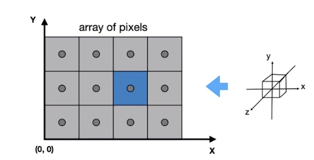
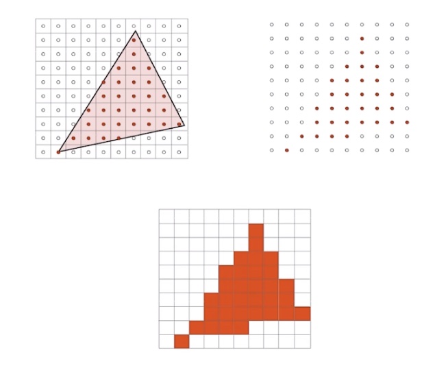
光栅化
- 把东西画在屏幕上
- 连续转离散
- 方法:采样
为什么不能直接使用投影变换?
投影变换中:
- 高斯核中心 \(x_k = [x_0, x_1, x_2]^\top\)
- 高斯核 \(r_k(x)=G_{v_k}(x-x_k)\)
- 均值 \(x_k = m(u_k)\),一个点,不会形变
- 协方差矩阵?透视投影到正交投影是非线性变换,即非仿射变换,但高斯椭球一直进行仿射变换,所以不能直接使用
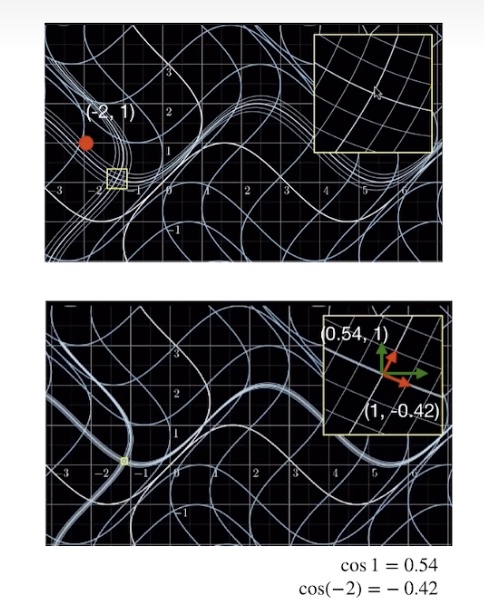
引入雅可比近似矩阵
- 泰勒展开、线性逼近
-
对非线性变换的局部线性近似
-
可计算得 \(J = \frac{\partial m(u_k)}{\partial u}\) 协方差矩阵 \(V_k = J V_k^\prime j^\top = JWV_k^{\prime \prime} W^\top J^\top\)
视口变换
此时均值和协方差在一个坐标系吗?
- 均值:在 NDC 坐标系 \([-1, 1]^3\),需要视口变换
- 协方差矩阵:在未缩放的正交坐标系 \([l,r] \times [b, t] \times [f, n]\),不需要视口变换
- 对于高斯核中心 \(\mu = [\mu_1, \mu_2, \mu_3]^\top\) 平移 + 缩放
- 对于协方差矩阵 足迹渲染:离散计算 \(G(\hat{x}) = \exp(-\frac{1}{2} (x-\mu)^\top V_k^{-1}(x-\mu))\)
3DGS 中心的变换 Code
# transform point, from world to ndc
# Notice, projmatrix already processed as mvp matrix
p_hom = transformPoint4x4(p_orig, projmatrix)
p_w = 1 / (p_hom[3] + 0.0000001)
p_proj = [p_hom[0] * p_w, p_hom[1] * p_w, p_hom[2] * p_w]

# transfrom point from NDC to Pixel
point_image = [ndc2Pix(p_proj[0], W), ndc2Pix(p_proj[1], H)]
3DGS 协方差矩阵的变换 Code
def computeCov2D(mean, focal_x, focal_y, tan_fovx, tan_fovy, cov3D, viewmatrix):
   # The following models the steps outlined by equations 29
   # and 31 in "EWA Splatting" (Zwicker et al., 2002).
   # Additionally considers aspect / scaling of viewport.
   # Transposes used to account for row-/column-major conventions.

   t = transformPoint4x3(mean, viewmatrix)

   limx = 1.3 * tan_fovx
   limy = 1.3 * tan_fovy
   txtz = t[0] / t[2]
   tytz = t[1] / t[2]
   t[0] = min(limx, max(-limx, txtz)) * t[2]
   t[1] = min(limy, max(-limy, tytz)) * t[2]

   J = np.array(
       [
           [focal_x / t[2], 0, -(focal_x * t[0]) / (t[2] * t[2])],
           [0, focal_y / t[2], -(focal_y * t[1]) / (t[2] * t[2])],
           [0, 0, 0],
       ]
   )
   W = viewmatrix[:3, :3]
   T = np.dot(J, W)

   cov = np.dot(T, cov3D)
   cov = np.dot(cov, T.T)

   # Apply low-pass filter
   # Every Gaussia should be at least one pixel wide/high
   # Discard 3rd row and column
   cov[0, 0] += 0.3
   cov[1, 1] += 0.3
   return [cov[0, 0], cov[0, 1], cov[1, 1]]
雪球颜色 球谐函数 
- 基函数:任何一个函数都可以分解为正弦核余弦的线性组合
- 球谐函数
- 任何一个球面坐标的函数都可以用多个球谐函数来近似
- \(f(t) \approx \sum_l \sum_{m=-l}^l c_l^m y_l^m (\theta, \phi)\)
- 其中,\(c_l^m\) 各项系数,\(y^m\) 基函数
- 论文中的 \(n=4\),共有 16 个参数(本质上是 1+3+5+7)
球谐函数 Code
def computeColorFromSH(deg, pos, campos, sh):
  # The implementation is loosely based on code for
  # "Differentiable Point-Based Radiance Fields for
  # Efficient View Synthesis" by Zhang et al. (2022)

  dir = pos - campos
  dir = dir / np.linalg.norm(dir)

  result = SH_C0 * sh[0]

  if deg > 0:
      x, y, z = dir
      result = result - SH_C1 * y * sh[1] + SH_C1 * z * sh[2] - SH_C1 * x * sh[3]

      if deg > 1:
          xx = x * x
          yy = y * y
          zz = z * z
          xy = x * y
          yz = y * z
          xz = x * z
          result = (
              result

              + SH_C2[0] * xy * sh[4]
              + SH_C2[1] * yz * sh[5]
              + SH_C2[2] * (2.0 * zz - xx - yy) * sh[6]
              + SH_C2[3] * xz * sh[7]
              + SH_C2[4] * (xx - yy) * sh[8]
          )

          if deg > 2:
              result = (
                  result

                  + SH_C3[0] * y * (3.0 * xx - yy) * sh[9]
                  + SH_C3[1] * xy * z * sh[10]
                  + SH_C3[2] * y * (4.0 * zz - xx - yy) * sh[11]
                  + SH_C3[3] * z * (2.0 * zz - 3.0 * xx - 3.0 * yy) * sh[12]
                  + SH_C3[4] * x * (4.0 * zz - xx - yy) * sh[13]
                  + SH_C3[5] * z * (xx - yy) * sh[14]
                  + SH_C3[6] * x * (xx - 3.0 * yy) * sh[15]
              )
  result += 0.5
  return np.clip(result, a_min=0, a_max=1)
为什么球谐函数能更好地表达颜色?
- 正常使用的 RGB 只有三个变量表达
- 球谐函数有 \(16 \times 3\) 个变量表达
足迹合成
- 直观上进行 \(\alpha\)-blending
- 实际上 3DGS 依然对每个像素着色,参考 NeRF 对光线上粒子进行求和
splatting 没有像 NeRF 一样找粒子的过程
- 对高斯球按照深度 z 排序,渲染的时候扔的顺序有关
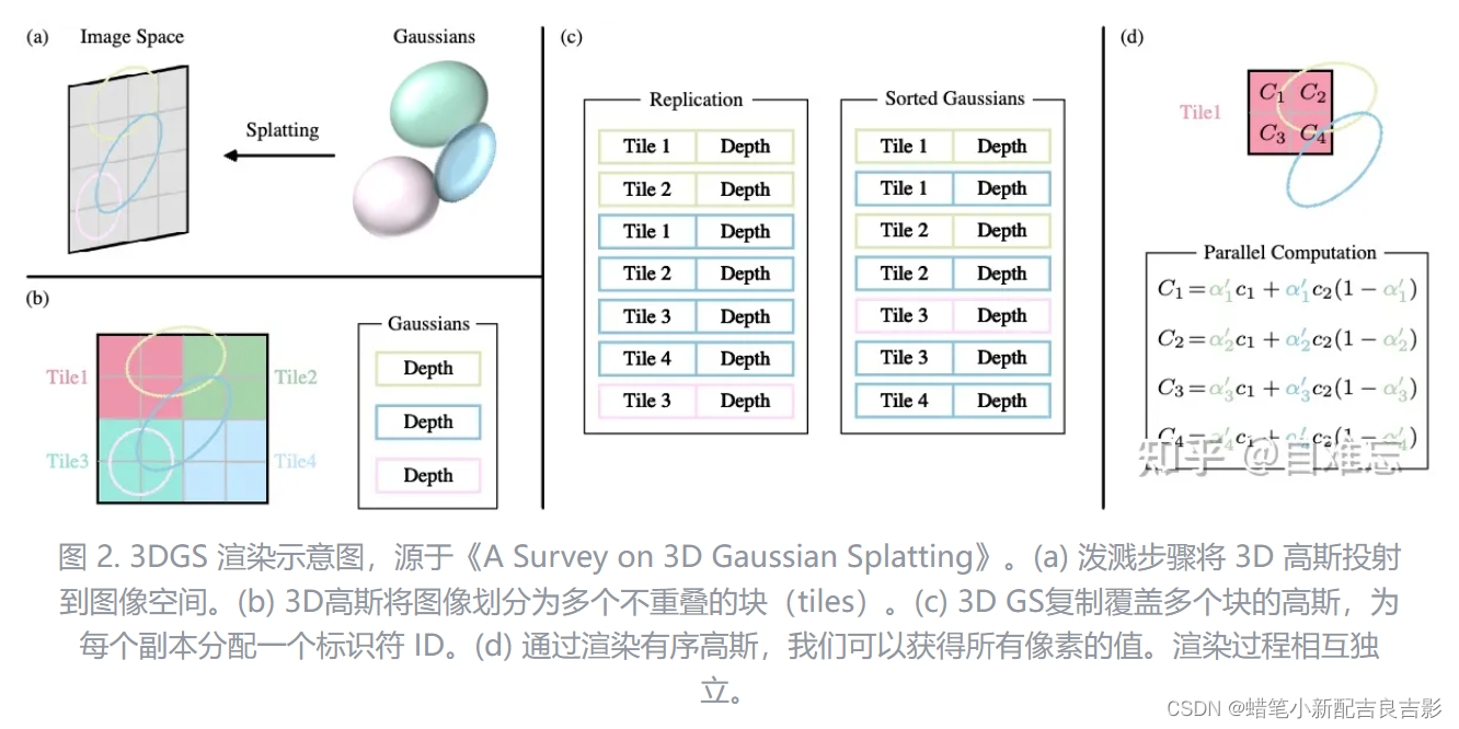
快速高斯光栅化 
延续 Splatting,如何快速高斯光栅化?
- 从像素级别的操作理解渲染过程:对于给定坐标 \(x\) 的像素点,可以通过视图变化计算出所有在该位置重叠的高斯的深度并排序,最后对排列好的高斯进行 \(\alpha\)-blending,返回该像素点最后的颜色值
\[
C = \sum_{i \in N} c_i \alpha^\prime \prod_{j=1}^{i-1}(1 - \alpha_j^\prime)
\]
由于排序过程难以并行化,3dgs 使用一些策略提高效率
- 使用图像块来代替像素级别的精度,每个块包含 \(16 \times 16\) 个像素,对于覆盖多个块的高斯,作者复制高斯并为它们分配标识符
- 每个块独立排序并计算颜色值,可并行执行
自适应高斯密度控制 
初始化的点云的初始形状是一个球,强依赖 SfM 生成的初始点云,可能导致生成高斯在空间密度过大或过小?
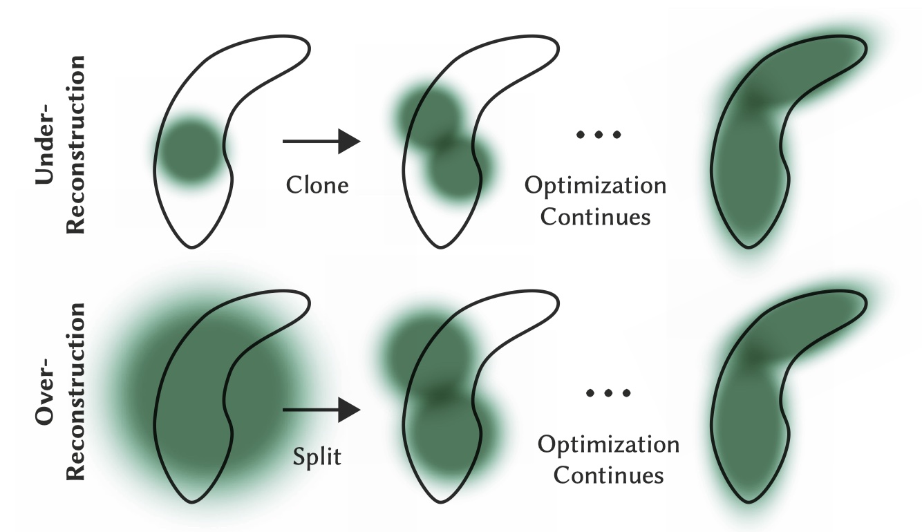
具体方法有点密集化和点剪枝。
点密集化 
- 重建不足的区域克隆小高斯
- 根据梯度的阈值条件和点云的缩放因子,生成一个选择点的掩码
selected_pts_mask - 基于选择的点生成新的点云坐标、特征、不透明度、缩放和旋转
- 将新生成的点云和特征附加到原始点云中
- 调用
densification_postfix函数对点云进行后处理
- 根据梯度的阈值条件和点云的缩放因子,生成一个选择点的掩码
densify_and_clone Code
def densify_and_clone(self, grads, grad_threshold, scene_extent):
    # Extract points that satisfy the gradient condition
    selected_pts_mask = torch.where(torch.norm(grads, dim=-1) >= grad_threshold, True, False)
    selected_pts_mask = torch.logical_and(selected_pts_mask,
                                          torch.max(self.get_scaling, dim=1).values <= self.percent_dense*scene_extent)

    new_xyz = self._xyz[selected_pts_mask]
    new_features_dc = self._features_dc[selected_pts_mask]
    new_features_rest = self._features_rest[selected_pts_mask]
    new_opacities = self._opacity[selected_pts_mask]
    new_scaling = self._scaling[selected_pts_mask]
    new_rotation = self._rotation[selected_pts_mask]

    self.densification_postfix(new_xyz, new_features_dc, new_features_rest, new_opacities, new_scaling, new_rotation)
- 重建过度的区域拆分大高斯
- 获取初始点云的数量
n_init_points - 创建一个与梯度相同大小的零张量
padded_grad,并将梯度值填充到其中 - 根据梯度的阈值条件和点云的缩放因子,生成一个选择点的掩码
selected_pts_mask - 将满足条件和缩放条件的点复制
N次,并计算新的坐标、缩放、旋转和特征 - 将新生成的点云和特征附加到原始点云
- 创建一个用于剪枝的过滤器
prune_filter,其中包括原始点云和新生成点云的掩码 - 根据剪枝过滤器删除不需要的点
- 获取初始点云的数量
densify_and_split Code
def densify_and_split(self, grads, grad_threshold, scene_extent, N=2):
    n_init_points = self.get_xyz.shape[0]
    # Extract points that satisfy the gradient condition
    padded_grad = torch.zeros((n_init_points), device="cuda")
    padded_grad[:grads.shape[0]] = grads.squeeze()
    selected_pts_mask = torch.where(padded_grad >= grad_threshold, True, False)
    selected_pts_mask = torch.logical_and(selected_pts_mask,
                                          torch.max(self.get_scaling, dim=1).values > self.percent_dense*scene_extent)

    stds = self.get_scaling[selected_pts_mask].repeat(N,1)
    means =torch.zeros((stds.size(0), 3),device="cuda")
    samples = torch.normal(mean=means, std=stds)
    rots = build_rotation(self._rotation[selected_pts_mask]).repeat(N,1,1)
    # 新生成点云信息(由大高斯分割并按一定系数缩放得到)
    new_xyz = torch.bmm(rots, samples.unsqueeze(-1)).squeeze(-1) + self.get_xyz[selected_pts_mask].repeat(N, 1)
    new_scaling = self.scaling_inverse_activation(self.get_scaling[selected_pts_mask].repeat(N,1) / (0.8*N))
    new_rotation = self._rotation[selected_pts_mask].repeat(N,1)
    new_features_dc = self._features_dc[selected_pts_mask].repeat(N,1,1)
    new_features_rest = self._features_rest[selected_pts_mask].repeat(N,1,1)
    new_opacity = self._opacity[selected_pts_mask].repeat(N,1)

    self.densification_postfix(new_xyz, new_features_dc, new_features_rest, new_opacity, new_scaling, new_rotation)

    prune_filter = torch.cat((selected_pts_mask, torch.zeros(N * selected_pts_mask.sum(), device="cuda", dtype=bool)))
    # 裁剪过程参照其不透明度值进行,裁剪掉不必要的点提高效率
    self.prune_points(prune_filter)
点剪枝 
- 将不透明度小于一定阈值的点减去,将过大的也减去,类似于正则化过程。并且在迭代一定次数后,高斯会被设置为几乎透明。这样就能有控制地增加必要的高斯密度,同时剔除多余的高斯。
- 根据最小不透明度和最大屏幕尺寸等条件生成剪枝掩码
prune_mask,并调用prune_points函数进行点云的剪枝操作 prune_points函数根据给定的掩码mask对点云进行剪枝操作,将不需要的点从点云中删除,并更新相关的张量数据
- 根据最小不透明度和最大屏幕尺寸等条件生成剪枝掩码
densify_and_prune Code
def densify_and_prune(self, max_grad, min_opacity, extent, max_screen_size):
    grads = self.xyz_gradient_accum / self.denom
    grads[grads.isnan()] = 0.0
    # 点密集化过程
    self.densify_and_clone(grads, max_grad, extent)
    self.densify_and_split(grads, max_grad, extent)

    prune_mask = (self.get_opacity < min_opacity).squeeze()
    if max_screen_size:
        big_points_vs = self.max_radii2D > max_screen_size
        big_points_ws = self.get_scaling.max(dim=1).values > 0.1 * extent
        prune_mask = torch.logical_or(torch.logical_or(prune_mask, big_points_vs), big_points_ws)
    self.prune_points(prune_mask)

    torch.cuda.empty_cache()

def prune_points(self, mask):
    valid_points_mask = ~mask
    optimizable_tensors = self._prune_optimizer(valid_points_mask)

    self._xyz = optimizable_tensors["xyz"]
    self._features_dc = optimizable_tensors["f_dc"]
    self._features_rest = optimizable_tensors["f_rest"]
    self._opacity = optimizable_tensors["opacity"]
    self._scaling = optimizable_tensors["scaling"]
    self._rotation = optimizable_tensors["rotation"]

    self.xyz_gradient_accum = self.xyz_gradient_accum[valid_points_mask]

    self.denom = self.denom[valid_points_mask]
    self.max_radii2D = self.max_radii2D[valid_points_mask]
参数估计 
- 初始点云,每个点膨胀成 3d 高斯椭球
- 则每个椭球的参数有:
- 中心点位置 \((x,y,z)\)
- 协方差矩阵 \(R,S\)
- 球谐函数系数 \(16 \times 3\)
- 透明度 \(\alpha\)
Source Code Review
学习自 学习笔记之——3D Gaussian Splatting 源码解读 _gaussian splatting 源码分析 -CSDN 博客
Experiment
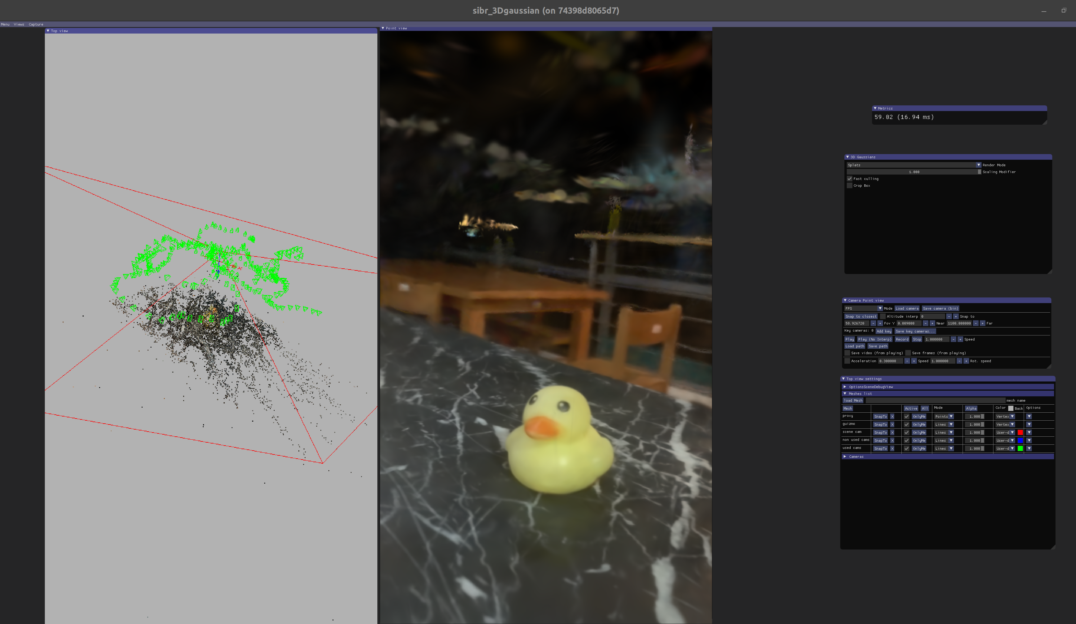
硬件配置
- Ubuntu 20.04 + 4060Ti + CUDA 11.8
- 跑在 Docker 11.8.0-cudnn8-devel-ubuntu22.04(镜像)
Office Scenes
Own Scenes
Reference
- 3D GaussianSplatting 技术的影响会有多大?
- 【较真系列】讲人话 -3d gaussian splatting 全解 ( 原理 + 代码 + 公式 )
- 3D Gaussian Splatting 原理速通
- 哈工大博士分享:基于 Gaussian Splatting 的 SLAM 新发展与新论文(上)
- 哈工大博士分享:基于 Gaussian Splatting 的 SLAM 新发展与新论文(下)
- (干货
) 《雅可比矩阵是什么东西》3Blue1Brown,搬自可汗学院。 【自制中文字幕】 - 学习笔记之——3D Gaussian Splatting 源码解读
- 3dgs_ 蜡笔小新配吉良吉影的博客 -CSDN 博客
- (三维重建学习)3D Gaussian Splatting & Instant-NGP 环境配置 _3d gaussian splatting 环境搭建 -CSDN 博客
- Gaussian Splatting 代码安装部署(windows)_gaussian splatting github-CSDN 博客
- 3D Gaussian Splatting 入门指南 - 哔哩哔哩